
2022 Stonk thoughts#
Itafos#
analysis can be performed better here.
Itafos stock valued about slightly above 3 PE. Given general food shortages and high fertilizer prices, would expect the value here to stay, even alternative producers like earth renew are going to need phosphate rock.
With market downturn, its possible this stock will go to 2 or 1 PE, net debt is acceptable.
They expect a slowing in H2 2022 as no one has money anymore.
Decent amount of shareholder equitity
214414000 USD, market cap
jun22_equitity = 214414	* 1000
# market cap in usd
market_cap =363.735 * 1000 * 1000

# ratio is
ratio = jun22_equitity / market_cap
print(ratio)
0.5894786039286843
So if the business is liquidized at the current price, 0.5 is returned to shareholders.
Earning back entire market cap in 2 or 3 years is appealing.
import matplotlib.pyplot as plt
plt.plot([100, 80, 75, 76, 85])
[<matplotlib.lines.Line2D at 0x7f084ff27d90>]
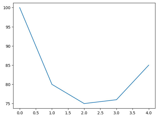
Earning should be sustained for a bit.
Plot of expected earnings over the next few years based on article of expected phosphate rock.
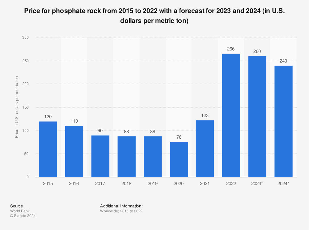
Find more statistics at Statista
ZIM#
I believe with the current supply chain issues, the inability to use rivers to ship goods, think container shipping is here to stay, port congestion is unlikely to end anytime soon with all the port strikes. Think zim will be able to maintain revenue for a few years.

Find more statistics at Statista
Seems like a lot of ships are old, think lifespan time is like 20 years, possible shipping remains high for a bit longer. With the aging fleet, I think https://gcaptain.com/old-is-gold-sky-high-cost-of-ageing-ships-sounds-inflation-sos/ and with supply chain issues with pretty high https://data.worldbank.org/indicator/IS.SHP.GOOD.TU shipping teu, makes sense that zim will be able to maintain high profits. Although the amount of teu went down in 2008, it was still high in recession, the rate may get lower, but I think zim will continue to deliver profits.
import matplotlib.pyplot as plt
# income for each quarter
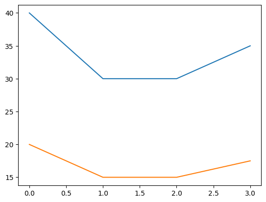
net_income = [40, 30, 30, 35]
plt.plot(net_income)
profit = [0.5 * income for income in net_income]
plt.plot(profit)
# with current profits I would expect
dividends = 20 + 15 + 15 + 17.5
ships last 20 or 25 years
Should get my money back in 2 to 3 years, dont expect shipping profits to collapse, new ships, environmental changes and climate change should keep profits high, and we are shipping more things than ever before.
Generates Record Full Year Net Income of $524 Million, in 2020 before the supply chain issues
import yfinance as yf
import mplfinance as mpf
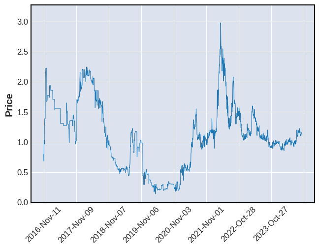
sp = yf.Ticker("MBCF")
# Consider grabbing for valid date index instead
daily = sp.history(start="2016-01-02")
mpf.plot(daily,type='line')
last_year = sp.history(start="2021-03-14")
mpf.plot(last_year,type='candle',mav=(50, 100),volume=True)
/opt/hostedtoolcache/Python/3.10.15/x64/lib/python3.10/site-packages/mplfinance/_arg_validators.py:84: UserWarning:

 =================================================================

   WARNING: YOU ARE PLOTTING SO MUCH DATA THAT IT MAY NOT BE
            POSSIBLE TO SEE DETAILS (Candles, Ohlc-Bars, Etc.)
   For more information see:
   - https://github.com/matplotlib/mplfinance/wiki/Plotting-Too-Much-Data

   TO SILENCE THIS WARNING, set `type='line'` in `mpf.plot()`
   OR set kwarg `warn_too_much_data=N` where N is an integer
   LARGER than the number of data points you want to plot.

 ================================================================
  warnings.warn('\n\n ================================================================= '+
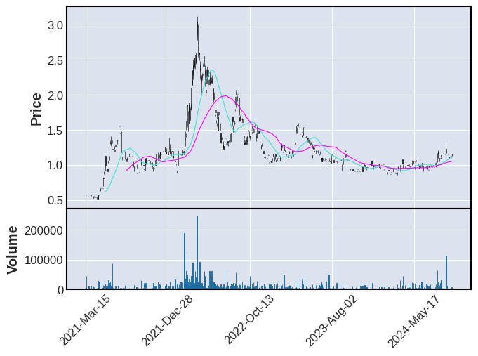
Its a bit above the 50MA, want to wait until its below.
Expect the bullwhip effect to happen a few times.
import numpy as np
def relative_strength(prices, n=14):
"""
compute the n period relative strength indicator
http://stockcharts.com/school/doku.php?id=chart_school:glossary_r#relativestrengthindex
http://www.investopedia.com/terms/r/rsi.asp
"""
deltas = np.diff(prices)
seed = deltas[:n + 1]
up = seed[seed >= 0].sum() / n
down = -seed[seed < 0].sum() / n
rs = up / down
rsi = np.zeros_like(prices)
rsi[:n] = 100. - 100. / (1. + rs)
for i in range(n, len(prices)):
delta = deltas[i - 1] # cause the diff is 1 shorter
if delta > 0:
upval = delta
downval = 0.
else:
upval = 0.
downval = -delta
up = (up * (n - 1) + upval) / n
down = (down * (n - 1) + downval) / n
rs = up / down
rsi[i] = 100. - 100. / (1. + rs)
return rsi
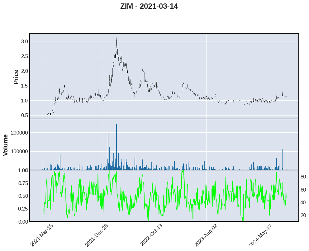
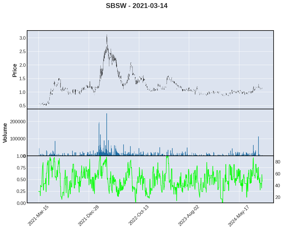
for stock in ["ZIM", "DOLE", "SBSW"]:
zim = yf.Ticker(stock)
zim = sp.history(start="2021-03-14")
zim['rsi'] = relative_strength(zim['Close'],n=7)
apd = mpf.make_addplot(zim['rsi'],panel=2,color='lime',ylim=(10,90),secondary_y=True)
mpf.plot(zim,type='candle',volume=True,figscale=1.5,addplot=apd,panel_ratios=(1,0.6), title=f"{stock} - 2021-03-14")
/opt/hostedtoolcache/Python/3.10.15/x64/lib/python3.10/site-packages/mplfinance/_arg_validators.py:84: UserWarning:

 =================================================================

   WARNING: YOU ARE PLOTTING SO MUCH DATA THAT IT MAY NOT BE
            POSSIBLE TO SEE DETAILS (Candles, Ohlc-Bars, Etc.)
   For more information see:
   - https://github.com/matplotlib/mplfinance/wiki/Plotting-Too-Much-Data

   TO SILENCE THIS WARNING, set `type='line'` in `mpf.plot()`
   OR set kwarg `warn_too_much_data=N` where N is an integer
   LARGER than the number of data points you want to plot.

 ================================================================
  warnings.warn('\n\n ================================================================= '+
Analyze of rollover of XSB, basic facts
2.74 years which is about 2 years and 8.2 months.
Current price 25.72, I am betting once the weak bonds expire, average bond yield at 0.61 %, reinvesting will result in a solid long term yield above the exist values. Assume current yield is rolling from 3 to 4.
TODO make model I can generalize
nav = 3282292855

current_yield = 2.24
# average bond yield for 2.74 years
lower_end = 3.25
higher_end = 4.5
avg_yield_for_years = 0.61

# assuming interest rates remain high for about 2.74 years
adjusted_yield_low =  ((lower_end / avg_yield_for_years)-current_yield*0.5) + current_yield * 0.5
adjusted_yield_high = ((higher_end / avg_yield_for_years)-current_yield*0.5) + current_yield * 0.5

# current rates are
print(adjusted_yield_low)


print(adjusted_yield_high)
# 5.327868852459017
# 7.377049180327869
5.327868852459017
7.377049180327869
Scenario for 0.75 0.25, 0.25 rate increases.
import pandas as pd
df = pd.read_csv("static_2019_to_now_boc_rates.csv")
last_date_in_csv = "2022-09-20"
first_hike = "2022-10-26"
base_rate = 3.25;
second_hike = "2022-12-07"
last_hike = "2023-01-26"

# list of objects, start, end, rate
future_date = "2023-11-25"
# create loop for this in the future
df['Date'] = pd.to_datetime(df['Date'])
to_first_hike = pd.DataFrame({'Date': pd.date_range(start=last_date_in_csv, end=first_hike,closed='left'), 'V39079': base_rate})

df.append(to_first_hike)
new_df = pd.concat([df, to_first_hike])
base_rate = base_rate + 0.75
to_second_hike = pd.DataFrame({'Date': pd.date_range(start=first_hike, end=second_hike,closed='left'), 'V39079': base_rate})

# have to draw rolling average with plot
new_df = pd.concat([new_df, to_second_hike])
base_rate = base_rate + 0.25
to_third_hike = pd.DataFrame({'Date': pd.date_range(start=second_hike, end=last_hike), 'V39079': base_rate})
new_df = pd.concat([new_df, to_third_hike])

to_future = pd.DataFrame({'Date': pd.date_range(start=last_hike, end=future_date), 'V39079': base_rate})
new_df = pd.concat([new_df, to_future])
to_future = pd.DataFrame({'Date': pd.date_range(start=future_date, end="2024-05-05"), 'V39079': base_rate-0.75})
new_df = pd.concat([new_df, to_future])
new_df = new_df[pd.to_numeric(new_df['V39079'], errors='coerce').notnull()]
# drop duplicates based on date
new_df = new_df.drop_duplicates()
# drop all zero entries

new_df["Rates"] = pd.to_numeric(new_df["V39079"])
new_df= new_df[new_df['Rates'] != 0]
# sort by Date
new_df.sort_values(by='Date', inplace=True)
# plot rolling average
new_df['MA'] = new_df["Rates"].rolling(600, min_periods=1).mean()
new_df.plot("Date", "Rates")
new_df.plot("Date", "MA")
print(new_df)
---------------------------------------------------------------------------
TypeError                                 Traceback (most recent call last)
Cell In[7], line 13
     11 # create loop for this in the future
     12 df['Date'] = pd.to_datetime(df['Date'])
---> 13 to_first_hike = pd.DataFrame({'Date': pd.date_range(start=last_date_in_csv, end=first_hike,closed='left'), 'V39079': base_rate})
     15 df.append(to_first_hike)
     16 new_df = pd.concat([df, to_first_hike])

File /opt/hostedtoolcache/Python/3.10.15/x64/lib/python3.10/site-packages/pandas/core/indexes/datetimes.py:1008, in date_range(start, end, periods, freq, tz, normalize, name, inclusive, unit, **kwargs)
   1005 if freq is None and com.any_none(periods, start, end):
   1006     freq = "D"
-> 1008 dtarr = DatetimeArray._generate_range(
   1009     start=start,
   1010     end=end,
   1011     periods=periods,
   1012     freq=freq,
   1013     tz=tz,
   1014     normalize=normalize,
   1015     inclusive=inclusive,
   1016     unit=unit,
   1017     **kwargs,
   1018 )
   1019 return DatetimeIndex._simple_new(dtarr, name=name)

TypeError: DatetimeArray._generate_range() got an unexpected keyword argument 'closed'
So this fails to account for proper weighting, accounting for high yield corporate bonds and heavily assumes that a lot of the debt will roll off successfully.
Assumes raises in government bonds will transfer over to the private sector (true, but companies may not be able to pay)
Assumes assets will roll over (true, but some may not), and greatly increase the yield, at bare minimum over a 2.74 year period would expect the yield to meet at least the benchmark yield, if not slightly higher.
import pandas as pd

df = pd.read_csv("xsb_holdings.csv")

# find columns with Duration less than 2 years and coupon less than 1.5%
df = df[(df["Duration"] < 2.74)]

print(df)

# total weight

print(df["Weight (%)"].sum())
print(df["Coupon (%)"].mean())
coupon_low = df[(df["Coupon (%)"] < 3)]
print(coupon_low["Coupon (%)"].mean())
print(coupon_low["Weight (%)"].sum())